# data
# abundance: normalised abundance matrix that was used for NMF
# W: matrix of genera weights in ES, obtained from NMF
# H: matrix of ES weights in samples, obtained from NMF
# model fit function (cosine similarity)
modelfit <- function(x, y) { x %*% y / sqrt(x%*%x * y%*%y) } # value of 1 = identical vectors
# reconstruct abundance matrix from W and H
reconstructed = W %*% H
# general model ft of the matrix
fit <- modelfit(c(reconstructed), c(abundance))
# sample-wise model fit
sample_fit <- c()
for (sample in colnames(abundance)){
sample_fit <- c(sample_fit, setNames(modelfit(reconstructed[, sample], abundance[,sample]), sample))
}
What are Enterosignatures?
Enterosignatures (ES) serve to break down the complexity of taxa in the gastrointestinal tract into generalizable characteristics that are valid across studies and enable accessible medical research. To identify these generalizable features from gut microbial profiles, we conducted a meta-analysis of 5,230 fecal metagenomes from 22 public studies. By applying non-negative matrix factorization (NMF) to the relative abundances of genera, we were able to reveal recurrent signatures from these profiles. We applied a 3x3 bi-cross validation to avoid overfitting and ensure there is a balance between explained microbial variance in the original dataset and applicability to new data.
Overview
On GitLab you can find the scripts for:
- Computing NMF on the whole dataset (enterosignatures_nmf.py)
- 9-fold bicross-validation (bicv_rank.py, bicv_regu.py)
- Applying existing ES on a new matrix (prepare_matrices.R, reapply_nmf.py)
Here you will also find more detailed information on the scripts.
Principle of NMF
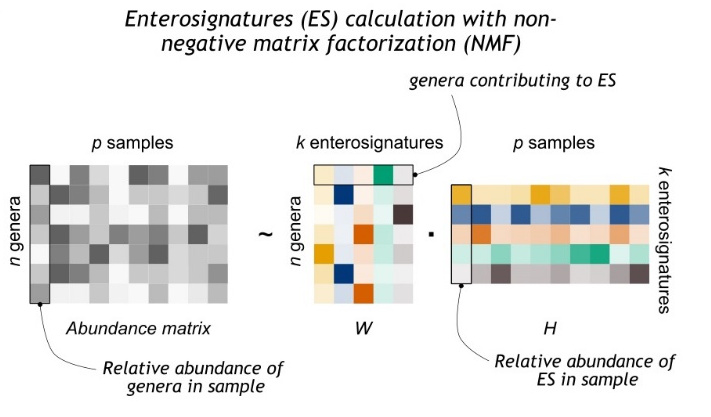
Calculation of Enterosignatures
The following workflow is described in more detail on GitLab.
- Normalize genus-level abundances per sample
- Calculate ES with NMF
- We used the function sklearn.decomposition.NMF from the scikit-learn package to perform the NMF.
- ES Analysis
- Normalize W and H matrices to get the weight of genera in ES and the relative abundances of ES in samples
- Calculate model fit score by sample
modelfit - function(x,y) { return (x %*% y / sqrt(x %*% x * y %*% * y)) } -
Visualize enterosignatures with the following Rscript:
library(ggplot2)
library(stringr)
library(gridExtra)

# W matrix is loaded and its rownames are set to the rownames of the original abundance matrix

# name the columns, ie the ES
es_names <- colnames(W_norm_byES) <- paste("ES", c(1:dim(W_norm_byES)[2]), sep = "_")

# normalize the W matrix by column, to get the relative abundance of genera in ES
W_norm_byES = sweep(W,2,colSums(W),"/")

# work with a data frame
dfw = as.data.frame(100*W_norm_byES)
dfw <-tibble::rownames_to_column(dfw, "tax")
# split the taxa ranks
dfw[c('kingdom', 'phylum', 'class', 'order', 'family', 'genus')] <- str_split_fixed(dfw$tax, ';', 6)

# set up a threshold of 3% for labelling of a genus in an ES
threshold <- 3
# prepare a list of plots
all_ES_plots <- list()

# loop over each ES to create individual barplots
for (es in es_names){
# label the genera only if relative abundance is > 0.03
dfw[[paste0("label", "_", es)]] <- ifelse(dfw[[es]] > threshold, dfw$genus, "")
# set up the max y value
maxy <- max(dfw[[es]])+0.1*max(dfw[[es]])
# main plot
p <- ggplot(dfw, aes_string(x="tax", y=es, fill="phylum")) +
geom_bar(stat="identity") +
labs(x="Genus", fill="Phylum") +
theme_classic() +
ylim(0, maxy) +
theme(panel.grid = element_blank(),
axis.title.x = element_blank(),
axis.line.x = element_blank(),
axis.text.x = element_blank(),
legend.position = "right",
panel.border = element_rect(colour = "black", fill=NA),
axis.text=element_text(size=10),
axis.ticks.x = element_blank(),
legend.text=element_text(size=8),
legend.title=element_text(size=8),
axis.title=element_text(size=10),
strip.text.x=element_text(size=10)
) +
geom_hline(yintercept = threshold, linetype="dashed", color="#DCDCDC") +
geom_text(aes(label = .data[[paste0("label", "_", es)]]), vjust = 0, angle = 15, hjust = 0, size = 2.5)
# enable text to superimpose outside the plot area
gg_table <- ggplot_gtable(ggplot_build(p + ggtitle(gsub("_", "-", es, perl = TRUE)) + labs(y="Relative ES composition (%)")))
gg_table$layout$clip[gg_table$layout$name=="panel"] <- "off"
grid.draw(gg_table)
# add the plot to the list
all_ES_plots[[es]] <- gg_table
}

# in order to visualize the plots, use grid.draw()
grid.draw(all_ES_plots$ES_1)
- 9-Fold bicross validation:
- Find the number of ES best fitting the dataset
The following code describes how to create the Enterosignature visualisation:
Applying existing ES to a new dataset
Existing ES can be applied to a new dataset by using a new normalized abundance matrix and an existing Weight-matrix to get the weight of the given ES in the new matrix. This is done with skilearn.decomposition.non_negative_factorization. A script for this is available on GitLab (prepare_matrices.R, reapply_nmf.py, GitLab).
In practice, obtaining H requires solving a non-negative least-square problem which can be done with the scikit-learn NMF function. Both the abundance matrix and the weight-matrix should share the taxa (rows in M and W)
This means that an a priori step is needed.
- Taxa of W that are missing in H should be added (with 0)
- Taxa of M that are missing in W should be added (with 0)
- We used the GTDB taxonomy for the original ES. To remain compatible we recommend to use the same taxonomic system in follow up studies.